01
Unit 18 · 2 hrs
NumPy Arrays
Numerical Python — foundation of scientific computing
Why NumPy? Python lists are slow for math. NumPy arrays are stored as contiguous memory blocks (C-style), enabling vectorized operations that are 10–100× faster.
Creating Arrays
import numpy as np

np.array([1,2,3])           # from list → 1D array
np.array([[1,2],[3,4]])     # 2D array (matrix)
np.zeros((3,4))              # 3×4 zeros
np.ones((2,3))               # 2×3 ones
np.arange(0, 10, 2)          # [0,2,4,6,8]
np.linspace(0, 1, 5)         # 5 evenly spaced [0..1]
np.eye(3)                     # 3×3 identity matrix
np.random.rand(2,3)          # 2×3 random [0,1)
Array Attributes & Indexing
a = np.array([[1,2,3],[4,5,6]])
a.shape     # (2, 3)
a.ndim      # 2
a.dtype     # int64
a.size      # 6 (total elements)

a[0, 1]     # 2  (row 0, col 1)
a[1, :]     # [4,5,6]  (all of row 1)
a[:, 2]     # [3,6]    (all of col 2)
a[0:2, 1:3] # [[2,3],[5,6]]  (submatrix)

# Boolean indexing
a[a > 3]    # [4, 5, 6]
Array Operations
a = np.array([1,2,3])
b = np.array([4,5,6])

a + b        # [5, 7, 9]   element-wise
a * b        # [4, 10, 18] element-wise
a ** 2       # [1, 4, 9]
np.dot(a,b)  # 32  (dot product)
np.sum(a)    # 6
np.mean(a)   # 2.0
np.max(a)    # 3
a.reshape(3,1) # column vector
02
Unit 19 · 3 hrs
Universal Functions & Broadcasting
Universal Functions (ufuncs)
Ufuncs operate element-wise on arrays. They're implemented in C — much faster than Python loops.
# Math ufuncs
np.sqrt([4,9,16])   # [2., 3., 4.]
np.exp([1,2])        # [e, e²]
np.log([1,10,100])  # natural log
np.sin(np.pi/2)     # 1.0
np.abs([-1,-2,3])   # [1, 2, 3]
Broadcasting Rules
Broadcasting lets NumPy operate on arrays of different shapes without copying data.
| Rule | Description |
|---|---|
| 1 | If arrays differ in ndim, pad smaller shape with 1s on LEFT |
| 2 | Dimensions of size 1 are stretched to match the other |
| 3 | Sizes must match or be 1 — otherwise ValueError |
a = np.array([[1],[2],[3]])  # shape (3,1)
b = np.array([10,20,30])    # shape (3,)
a + b  # shape (3,3) — broadcasts both
# [[11,21,31],[12,22,32],[13,23,33]]
Fancy Indexing
a = np.array([10,20,30,40,50])
a[[0,2,4]]     # [10, 30, 50] — index with list
a[a > 25]      # [30, 40, 50] — boolean mask
a[a % 20 == 0] # [20, 40]
03
Unit 20 · 3 hrs
Pandas — Series & DataFrames
Pandas in simple words: Pandas helps you work with table-like data (like Excel sheets) in Python.
If NumPy is for fast numbers, Pandas is for real-world data with row names, column names, missing values, filtering, and summaries.
Series vs DataFrame (for beginners)
| Object | Think of it as | Shape | Example |
|---|---|---|---|
| Series | One labeled column | 1D | Ages of students |
| DataFrame | Full table (many columns) | 2D | Name + Age + Score table |
Memory trick: Series = single lane. DataFrame = full highway with many lanes.
Series
A Series is one column of data with labels (index). You can access values by label or by position.
import pandas as pd

# From list (default int index)
s = pd.Series([10,20,30])

# From dict (keys become index)
s = pd.Series({'a':10, 'b':20})
s['a']     # 10
s.values   # numpy array
s.index    # Index(['a','b'])
DataFrame
A DataFrame is a 2D table made of multiple Series sharing the same row index.
df = pd.DataFrame({
    'Name': ['Alice','Bob','Carol'],
    'Age':  [25, 30, 22],
    'Score':[88, 72, 95]
})

df.head(2)          # first 2 rows
df.shape            # (3, 3)
df.dtypes           # column types
df['Age']           # Series (column)
df[['Name','Score']] # sub-DataFrame
df.iloc[0]          # first row by position
df.loc[0, 'Name']   # label-based: 'Alice'
df[df['Score'] > 80]# filter rows
Key DataFrame Operations
| Operation | Code |
|---|---|
| Describe stats | df.describe() |
| Sort by column | df.sort_values('Age') |
| Group & aggregate | df.groupby('Dept')['Score'].mean() |
| Drop column | df.drop('Age', axis=1) |
| Handle missing | df.fillna(0) / df.dropna() |
| From CSV | pd.read_csv('file.csv') |
| To CSV | df.to_csv('out.csv', index=False) |
iloc vs loc:
iloc = integer position (0-based). loc = label-based (uses index labels). Mixing them up is a common bug.04
Unit 21 · 2 hrs
Matplotlib — Basic Plotting
import matplotlib.pyplot as plt

# Simple example: heights of students (bar chart)
students = ['Asha', 'Ben', 'Chen', 'Diya', 'Evan']
heights = [152, 160, 155, 167, 162]

plt.bar(students, heights)
plt.title('Heights of Students in a Class')
plt.xlabel('Student')
plt.ylabel('Height (cm)')
plt.show()
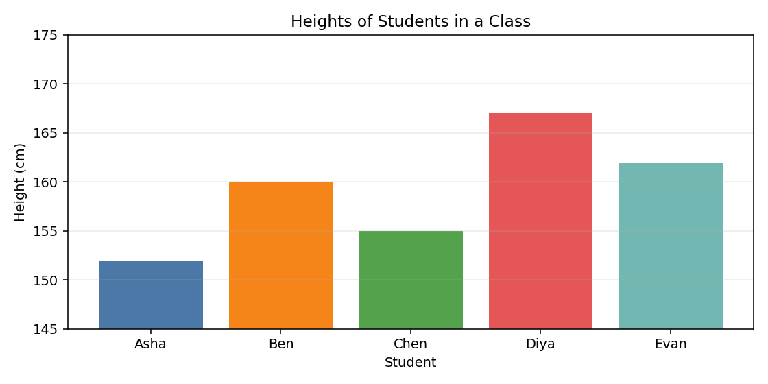
Chart Types
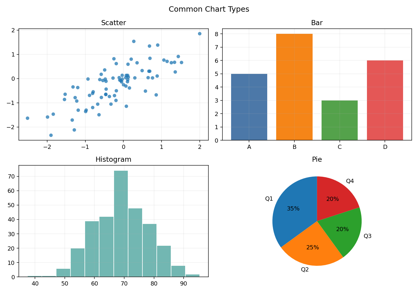
| Chart | Function | Use For |
|---|---|---|
| Line plot | plt.plot(x, y) | Trends over continuous x |
| Scatter plot | plt.scatter(x, y) | Correlation between two vars |
| Bar chart | plt.bar(categories, values) | Comparing discrete categories |
| Histogram | plt.hist(data, bins=10) | Distribution of a variable |
| Pie chart | plt.pie(sizes, labels=labels) | Proportions of a whole |
Subplots
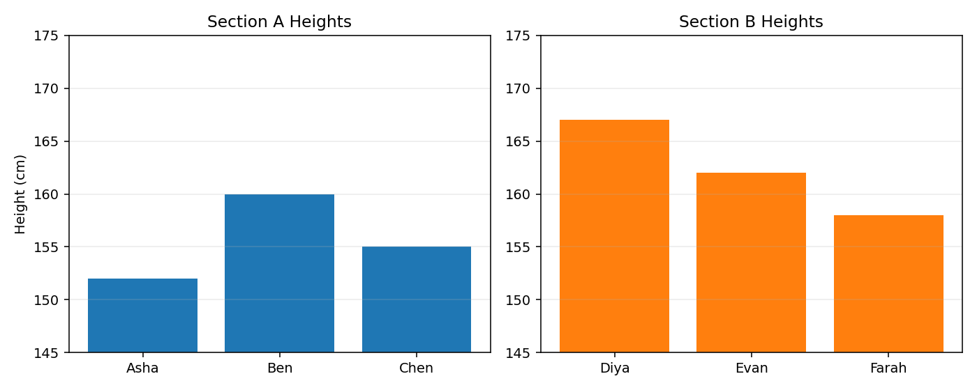
# Compare two class sections side-by-side
students_a = ['Asha', 'Ben', 'Chen']
heights_a = [152, 160, 155]

students_b = ['Diya', 'Evan', 'Farah']
heights_b = [167, 162, 158]

fig, axes = plt.subplots(1, 2, figsize=(10,4))
axes[0].bar(students_a, heights_a); axes[0].set_title('Section A Heights')
axes[1].bar(students_b, heights_b); axes[1].set_title('Section B Heights')
plt.tight_layout()
plt.show()
Always call
plt.show() last (in scripts). In Jupyter: use %matplotlib inline at the top.FC
Quick Review
Flashcards — Module IV
Tap to flip